Challenger Chicago stats & predictions

Upcoming Tennis Challenger Chicago: A Deep Dive into Tomorrow's Matches

The Tennis Challenger Chicago is set to captivate fans and enthusiasts with its upcoming matches. This prestigious event, known for showcasing emerging talents and seasoned players alike, promises an exhilarating day of tennis action. As we look ahead to tomorrow's matches, let's delve into the lineup, explore expert betting predictions, and analyze key players who could make a significant impact on the court.

Match Lineup and Key Players

Tomorrow's schedule is packed with thrilling encounters that will test the skills and strategies of the participating players. Here are some of the standout matches:

• Match 1: Player A vs. Player B
• Match 2: Player C vs. Player D
• Match 3: Player E vs. Player F

Taking Advantage of Live Streaming Options

If you can't make it to Chicago or prefer watching from home, live streaming offers an excellent alternative. Here’s how you can catch all the action live:

• Sports Streaming Services: Many services offer live streaming of tennis tournaments. Check out platforms like ESPN+, Tennis TV, or other sports networks that cover international events.
• Tournament Website: Visit the official Tennis Challenger Chicago website for potential links or information about live streams.
• Social Media Highlights: Even if full matches aren't streamed live, social media platforms often provide real-time highlights and key moments from each game.
• jimmy-lee-lee/ML-Notes<|file_sep|>/README.md # ML-Notes Notes from machine learning courses <|repo_name|>jimmy-lee-lee/ML-Notes<|file_sep|>/CS224d/Week1.md # Week1 ## Part1 - Introduction #### CS224d is focused on: * Neural network models that have been applied successfully or promisingly in NLP. * Notation used throughout course. #### Some popular NLP applications: * Machine Translation (MT) * Speech Recognition * Sentiment Analysis * Dialogue Systems #### Basic Idea behind Neural Networks * We want NNs that map input vectors x into output vectors y. * We do this by composing several simple functions f together. * We do this by composing several simple functions f together:  #### Some basic definitions * **Model**: a function f(x) that maps input vectors x into output vectors y. * **Parameters**: we use parameters θ (theta) instead of weights w because it is common in ML * **Loss function**: We measure how good our model is by comparing its output y_pred = f(x; θ) against some ground truth label y_true.  #### Optimization Objective  #### Feedforward Neural Networks  #### Notation used throughout course:  #### Backpropagation  ## Part2 - Word Embeddings ### Overview The goal is mapping words onto vectors (also called embeddings) such that similar words are mapped close together. We can use word embeddings as features for our models. ### Distributional Hypothesis Words that occur in similar contexts tend to have similar meanings. ### Word Embeddings vs One-hot encodings One-hot encodings: * One-hot encoding represents words as binary vectors where only one element is non-zero. * One-hot encodings are sparse (very inefficient) * One-hot encodings do not capture semantic similarities between words. Word Embeddings: * Word embeddings are dense real-valued vectors which represent words. * Word embeddings capture semantic similarities between words. ### Example application: Word Similarity Task Given two words w1,w2 find whether they are semantically similar or not. Example: python w1 = 'king' w2 = 'queen' We want a model which returns True since 'king' is semantically similar to 'queen'. ### Example application: Analogy Task Given three words w1,w2,w3 find word w4 such that w1:w2 = w3:w4. Example: python w1 = 'man' w2 = 'woman' w3 = 'king' We want a model which returns 'queen' since 'man' is related to 'woman' just like 'king' is related to 'queen'. ### Cosine Similarity Cosine similarity measures how similar two vectors are. It measures cosine of angle θ between two vectors x,y. Cosine similarity ranges from -1 (completely dissimilar) -> +1 (exactly same). Formally,  where x⋅y denotes dot product between x,y. ### Word Embedding Model We assume that each word wi corresponds with some vector v(wi). The probability that word wj occurs given word wi depends on cosine similarity between v(wi),v(wj). Formally,  where ||v|| denotes norm of vector v. ### Training Objective To learn word embedding parameters we need training data containing pairs (wi,wj). For example, python train_data = [('the', 'king'), ('the', 'queen'), ('the', 'prince')] The training objective is defined as follows:  where Z = Σk exp(v(wk)⋅v(wi)/||v(wk)|| ||v(wi)||). In other words, we want our model parameters such that probability of co-occuring word wj given word wi is maximized. ### Stochastic Gradient Descent (SGD) We define loss L(θ) = −log P(wj|wi; θ) where θ denotes model parameters. We then update our model parameters using SGD as follows:  where α >0 denotes learning rate. ### Negative Sampling (NS) **Problem**: NS reduces computational complexity from O(V) -> O(k) where V denotes vocabulary size while keeping quality almost same. **Solution**: Instead of computing denominator term Z we sample k "negative" samples wn from vocabulary V uniformly at random such that wn ≠ wi,wj ∀n. We then approximate Z by summing over k negative samples plus original positive sample (wj): Z ≈ exp(v(wj)⋅v(wi)/||v(wi)|| ||v(wj)||) + Σn=1k exp(v(wn)⋅v(wi)/||v(wn)|| ||v(wi)||). We then update our loss function as follows: L(θ) = −log P(wj|wi; θ) − Σn=1k log(1 − P(wn|wi; θ)). Note that we still use original positive sample (wj) but instead we use negative samples wn when computing denominator term Z so loss function becomes:  where P(wn|wi; θ) = σ(v(wn)⋅v(wi)/||v(wn)|| ||v(wi)||). We then update our model parameters using SGD as follows:  Note that we update parameters using both positive sample (wj) as well as negative samples wn.<|file_sep|># Week2 ## Part1 - Recurrent Neural Networks ### Motivation RNNs allow us process sequences of data such as sentences or music scores where input x_t depends on previous inputs x_0,x_1,...x_t−1 . In addition RNNs allow us work with variable length sequences unlike feedforward neural networks which require fixed length inputs. ### Overview RNNs work by maintaining an internal state h_t which summarizes information seen so far i.e., h_t depends on previous inputs x_0,x_1,...x_t−1 . The RNN then produces output y_t depending on current input x_t as well as internal state h_t . In other words, RNN maintains internal state h_t which summarizes information seen so far i.e., h_t depends on previous inputs x_0,x_1,...x_t−1 . The RNN then produces output y_t depending on current input x_t as well as internal state h_t . 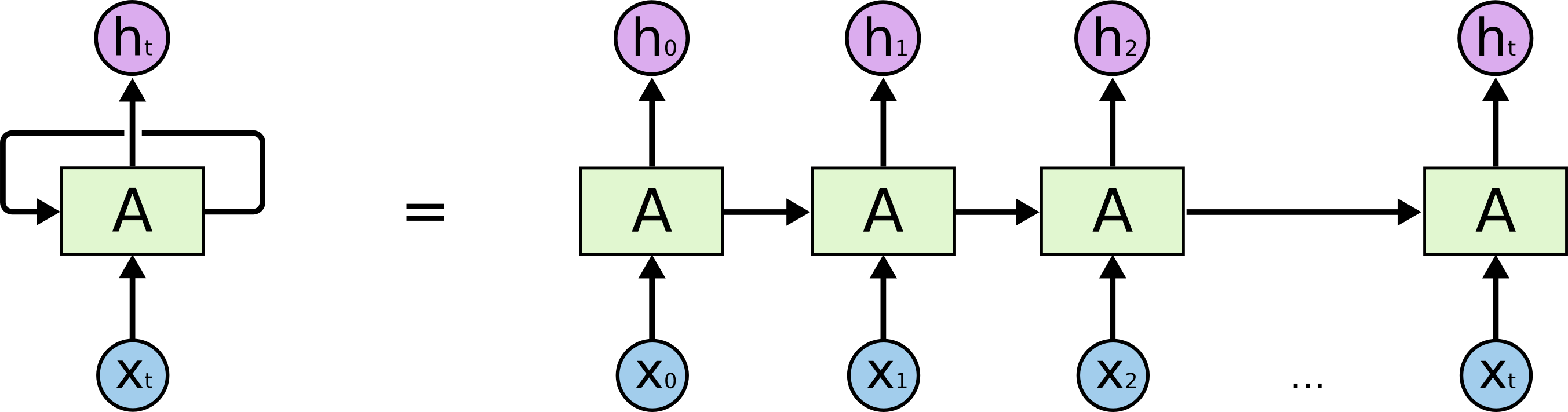Formally,  where g(.) denotes activation function such as tanh or ReLU . ### Example Application: Language Modeling Language modeling involves predicting next word given previous sequence of words i.e., given sentence "I went out yesterday" predict next word "for". We assume each word corresponds with some embedding vector v(w). Formally, Given sequence x_0,x_1,...x_T−1 find p(x_T |x_0,x_1,...x_T−1 ). If we use RNN then we set x_t=v(x_t). Then RNN computes internal states h_0,h_1,...h_T−1 . Finally we compute p(x_T |x_0,x_1,...x_T−1 )=softmax(Wx_T + U h_T−1+b). In other words, we first compute embedding vector v(x_t)=Vx_t+b_w for each input word x_t . Then we compute internal states h_0,h_1,...h_T−1 using RNN equation above . Finally we compute p(x_T |x_0,x_1,...x_T−1 )=softmax(Wx_T + U h_T−1+b). Formally,  where W,U,V,W,b_w,U,b_h,b_y denote model parameters . ### Training Objective To train our RNN language model we need training data consisting of sequences S=(S^m)_m=^M where S^m=(w^m_0,w^m_1,...w^m_L−m ) . For example, python train_data = [ 'She went out yesterday', 'He went out today', 'I went out yesterday', 'I am going out today' ] Our training objective consists in maximizing log probability over all sequences S∈train_data :  Formally,  where M denotes number of sequences , L_m denotes length of sequence m , W,S,T denote start/end tokens respectively , L denotes total number of tokens across all sequences , W_x,W_h,W_y,U,V,b_w,b_h,b_y denote model parameters , g(.) denotes activation function such as tanh or ReLU , softmax(.) denotes softmax activation function , p(.) denotes probability distribution . ### Backpropagation Through Time (BPTT) To train our RNN language model using SGD we need gradients ∂L/∂W_x , ∂L/∂W_h , ∂L/